Rehan Sheikh

Part of my role as CTO of Remade AI is working on diffusion models, the new generation of which are Latent Diffusion Models (LDMs). These models operate in a compressed latent space and VAEs are the things that do the "compressing" and "decompressing." An interesting byproduct of working with such models is that my cofounders have often found me in the office at 2am staring at the screen muttering to myself "What the F*** is a VAE?" This blog post is my attempt to answer that question!

What are Autoencoders?

An autoencoder is a type of neural network that learns to reconstruct its input data $\mathbf{x}$ . It has two main components:

Encoder ( $f_{\theta}$ ): Compresses $\mathbf{x} \in \mathbb{R}^d$ into a lower-dimensional latent representation $\mathbf{z} \in \mathbb{R}^k$ , where typically $k \ll d$ . $\mathbf{z} = f_{\theta}(\mathbf{x})$
Decoder ( $g_{\phi}$ ): Reconstructs (or "decodes") the latent vector $\mathbf{z}$ back into $\hat{\mathbf{x}}$ , an approximation of the original input. $\hat{\mathbf{x}} = g_{\phi}(\mathbf{z})$

Putting it all together, a forward pass through the autoencoder typically looks like:

\mathbf{x} \;\;\longrightarrow\;\; f_{\theta}(\mathbf{x}) \;=\; \mathbf{z} \;\;\longrightarrow\;\; g_{\phi}(\mathbf{z}) \;=\; \hat{\mathbf{x}}

During training, we want $\hat{\mathbf{x}}$ to be as close as possible to $\mathbf{x}$ . A common way to measure the difference between $\mathbf{x}$ and $\hat{\mathbf{x}}$ is through a mean squared error (MSE) loss:

\mathcal{L}_{\text{recon}}(\mathbf{x}, \hat{\mathbf{x}}) \;=\; \|\mathbf{x} \;-\; \hat{\mathbf{x}}\|^2

Hence, the autoencoder is typically trained by minimizing the sum of these reconstruction losses across all data points:

\min_{\theta, \phi} \;\sum_{i=1}^{N} \mathcal{L}_{\text{recon}}\!\Bigl(\mathbf{x}^{(i)}, \,\hat{\mathbf{x}}^{(i)}\Bigr)

where $\theta$ and $\phi$ are the parameters of the encoder and decoder, respectively, and $N$ is the number of training samples.

Because the latent dimension $k$ is strictly less than the input dimension $d$ , the network is forced to learn a compressed representation of the data. This process:

Encourages dimensionality reduction: The encoder-decoder structure is somewhat analogous to a learned, potentially nonlinear version of principal component analysis (PCA).
Extracts features: The latent code $\mathbf{z}$ often captures relevant factors of variation in the data.

However, classic autoencoders mainly focus on reconstruction and do not impose structure on $\mathbf{z}$ to enable generation of new data from scratch. To address this, we introduce a probabilistic perspective on the latent space in the variational autoencoder (VAE), ensuring a smoother and more meaningful latent distribution suitable for generative modeling.

Figure 1: Training visualization of an autoencoder on MNIST digits: Original images (top) and their reconstructions (bottom) are shown, along with the training loss curve over 100 epochs.

Variational Autoencoders (VAEs)

A variational autoencoder (VAE) can be understood as a latent variable model with a probabilistic framework over both observed data $\mathbf{x}$ and hidden (latent) variables $\mathbf{z}$ . Instead of deterministically mapping $\mathbf{x}$ to a single point $\mathbf{z}$ , a VAE places a distribution over $\mathbf{z}$ conditioned on $\mathbf{x}$ and imposes a prior distribution on $\mathbf{z}$ itself.

We assume our data $\mathbf{x}$ (e.g., images) are generated by a two-step probabilistic process:

\mathbf{z} \sim p(\mathbf{z}), \quad \mathbf{x} \sim p_{\theta}(\mathbf{x}\mid\mathbf{z})

where:

$p(\mathbf{z})$ is the prior over latent variables. Commonly, $p(\mathbf{z})$ is chosen to be a simple Gaussian $\mathcal{N}(\mathbf{0}, \mathbf{I})$ .
$p_{\theta}(\mathbf{x}\mid\mathbf{z})$ is the likelihood model (decoder), parameterized by $\theta$ (e.g., a neural network).

Hence, the joint distribution factorizes as:

p_{\theta}(\mathbf{x}, \mathbf{z}) \;=\; p_{\theta}(\mathbf{x}\mid \mathbf{z})\, p(\mathbf{z})

We are often interested in the posterior distribution $p(\mathbf{z}\mid\mathbf{x})$ , i.e. how the latent $\mathbf{z}$ is distributed once we have observed data $\mathbf{x}$ . By Bayes' rule:

p(\mathbf{z}\mid\mathbf{x}) \;=\; \frac{p_{\theta}(\mathbf{x}\mid\mathbf{z})\, p(\mathbf{z})}{p(\mathbf{x})}

but $p(\mathbf{x})$ (the evidence) involves an integral over all possible $\mathbf{z}$ :

p(\mathbf{x}) \;=\;\int p_{\theta}(\mathbf{x}\mid\mathbf{z}) \,p(\mathbf{z}) \,d\mathbf{z}

which is typically intractable for high-dimensional or richly-parameterized neural networks.

To circumvent this, we introduce a tractable approximation $q_{\phi}(\mathbf{z}\mid\mathbf{x})$ , where $\phi$ are the variational parameters (often another neural network, sometimes called the encoder). We want $q_{\phi}(\mathbf{z}\mid\mathbf{x})$ to be "as close as possible" to the true posterior $p_{\theta}(\mathbf{z}\mid\mathbf{x})$ .

A standard choice is to let $q_{\phi}(\mathbf{z}\mid\mathbf{x})$ be a Gaussian (e.g. $\mathcal{N}(\boldsymbol{\mu}(\mathbf{x}), \mathbf{\Sigma}(\mathbf{x}))$ ), whose mean and (diagonal) covariance come from a neural network.

Learning by Maximizing the Evidence Lower Bound (ELBO)

We define the variational lower bound (ELBO) on $\log p_{\theta}(\mathbf{x})$ :

\log p_{\theta}(\mathbf{x}) \;\;\ge\;\; \underbrace{\,\mathbb{E}_{q_{\phi}(\mathbf{z}\mid\mathbf{x})}\bigl[\log p_{\theta}(\mathbf{x}\mid \mathbf{z})\bigr] \;-\; D_{\mathrm{KL}}\!\bigl(q_{\phi}(\mathbf{z}\mid\mathbf{x}) \,\|\, p(\mathbf{z})\bigr)\,}_{\text{ELBO}(\theta,\phi,\mathbf{x})}

Thus, the VAE objective is:

\max_{\theta, \phi} \bigl\{\text{ELBO}(\theta, \phi)\bigr\} \;=\; \max_{\theta, \phi} \Bigl\{ \mathbb{E}_{q_{\phi}(\mathbf{z}\mid\mathbf{x})}\bigl[\log p_{\theta}(\mathbf{x}\mid\mathbf{z})\bigr] \;-\; D_{\mathrm{KL}}\!\bigl(q_{\phi}(\mathbf{z}\mid\mathbf{x}),\, p(\mathbf{z})\bigr) \Bigr\}

By optimizing this lower bound, we simultaneously:

Maximize reconstruction quality (the first term, $\mathbb{E}[\log p_{\theta}(\mathbf{x}\mid\mathbf{z})]$ )
Regularize the latent space (the second term, the KL divergence to a simple prior)

With a well-regularized latent space, we can sample new data by:

\mathbf{z}^{(\text{new})} \sim p(\mathbf{z}) \quad\Rightarrow\quad \hat{\mathbf{x}}^{(\text{new})} = p_{\theta}(\mathbf{x}\mid \mathbf{z}^{(\text{new})})

thus generating novel outputs in the data space. This property makes VAEs a powerful approach for generative modeling—each latent vector $\mathbf{z}^{(\text{new})}$ decodes into a coherent sample $\hat{\mathbf{x}}^{(\text{new})}$ .

Figure 2: Visualization of latent space interpolation in a VAE. Points

z_i

and

z_e

represent the initial and end states in the latent space, while

z_I

shows the current interpolation point. As

z_I

moves along the path between

z_i

and

z_e

, the decoder generates corresponding images, demonstrating smooth transitions between learned representations.

Disentangled VAEs (and Why We Care)

A disentangled variational autoencoder aims for each latent dimension (or a small subset thereof) to correspond to a single factor of variation in your dataset. In other words, we'd love each axis in $\mathbf{z}$ to capture a different interpretable property, for example line thickness or tilt, without mixing those properties in the same dimension.

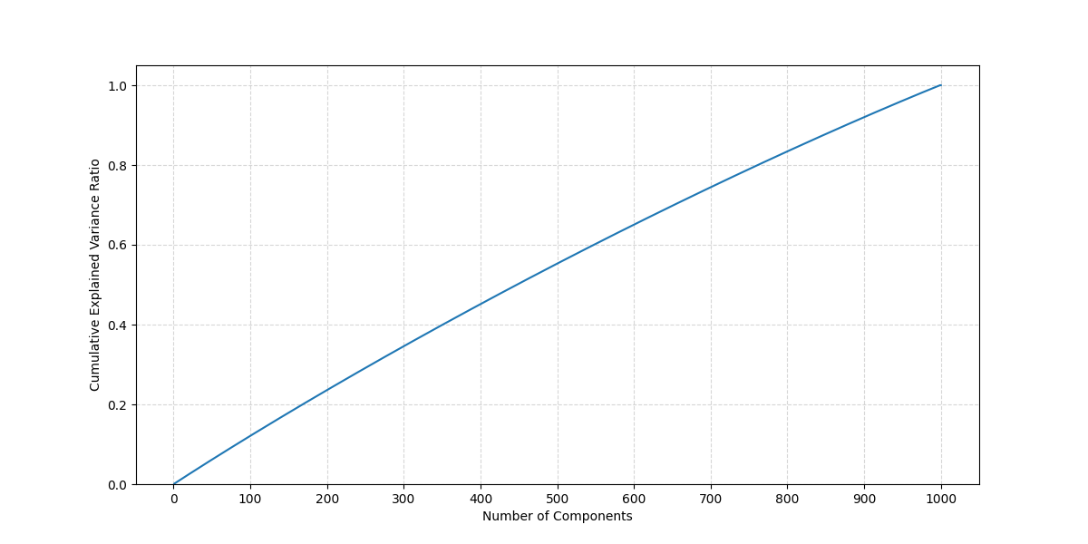
In an ideal disentangled latent space, we might see that a few principal axes explain most of the variance near an encoded point $\mathbf{z}_0$ . But in practice, the Flux VAE, we observe from Figure 3 that the cumulative explained variance follows a logarithmic-like climb, implying no single dimension (or handful of them) dominates.

Since the curve has no clear "elbow," it suggests these latent spaces are quite entangled e.g. the variance is spread out, with no single direction accounting for a big chunk of variation.

PCA explained variance ratio for FLUX VAE — **Figure 3:** Cumulative PCA explained variance for the *Flux VAE*. The curve shows a smooth, log-like rise—no single dimension stands out as a clear principal component.

To visualize whether certain directions in latent space produce coherent changes, we took the top 5 PCA components from that local neighborhood and stepped along each direction. Then, for each step in these directions, we decode back to image space.

The Flux VAE shows somewhat "random" or "flickering" transformations. In Figure 4 (the accompanying GIF), the reconstructions look mostly like noise or small chaotic changesindicating these latent directions do not correspond to a single factor (e.g., shape or color).

Figure 4: GIF stepping along top 5 PCA directions near an encoded image in the FLUX VAE, producing pseudo-random variation rather than a clear, single-factor transformation.

Conditioned Beta-VAE (on MNIST)

We can still find ways to achieve partial disentanglement, especially on simpler or labeled data. Below is an interactive demo of a Conditioned Beta-VAE trained on the MNIST dataset:

"Conditioned" means we feed the digit class label $y$ along with the image $\mathbf{x}$ into the encoder and decoder. This helps the VAE to separate label-driven variation from other variation.
"Beta" means we scale the KL term by $\beta$ , pushing the model to compress the representation more aggressively and (hopefully) isolate distinct factors in separate latent dims.

Mathematically, the Conditioned Beta-VAE modifies the usual VAE objective. If we denote the data-label pair as $(\mathbf{x}, y)$ , and the latent as $\mathbf{z}$ , we have:

\begin{aligned} \mathcal{L}_{\beta}(\theta, \phi) &= \mathbb{E}_{q_{\phi}(\mathbf{z} \mid \mathbf{x}, y)}\bigl[\log p_{\theta}(\mathbf{x}\mid \mathbf{z}, y)\bigr] \;-\; \beta \,\mathrm{KL}\!\Bigl( q_{\phi}(\mathbf{z}\mid \mathbf{x}, y) \;\|\; p(\mathbf{z}) \Bigr) \,. \end{aligned}

Here, $q_{\phi}(\mathbf{z}\mid \mathbf{x}, y)$ is the encoder distribution (mean & log-variance come from a neural net that sees both $\mathbf{x}$ and label $y$ ). Similarly, the decoder $p_{\theta}(\mathbf{x}\mid\mathbf{z}, y)$ can incorporate the class label as an additional input.

We set $\beta$ to some value > 1 to further encourage the distribution over $\mathbf{z}$ to stay close to a factorized Gaussian prior, yielding disentangled latents if the data factors are suitable.

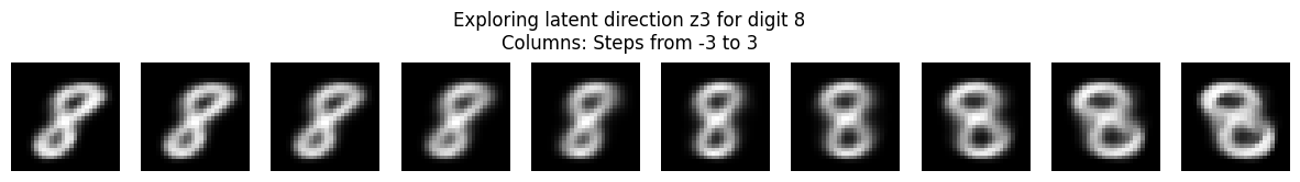
Varying dimension 3 of the latent space shows tilt variation — **Figure 5:** Varying dimension 3 of the latent vector shows clear tilt variation in the generated digits, while other attributes remain relatively constant.

The demo below runs entirely client-side using ONNX Runtime Web. I first trained the model in PyTorch, saved it as a safetensors checkpoint, then converted it to ONNX format using torch.onnx.export. The resulting ONNX model is loaded directly in the browser via onnxruntime-web, which provides efficient inference without any server calls. When you interact with the demo, dimension #3 of the latent space shows clear control over the digit's tilt - a nice example of disentanglement!

Adjusting $\mathbf{z}_3$ dimension

Value: 0.0

Figure 6: Interactive Conditioned Beta-VAE on MNIST. You can pick a digit label and vary dimension #3 of

\mathbf{z}

, which rotates the digit. One dimension, one factor.

Disentangled Latent Spaces and Diffusion Models

Latent diffusion models (LDMs) run the diffusion process in a compressed latent space rather than raw pixels. If that latent space is disentangled, the diffusion process can manipulate distinct factors more easily. For instance:

The diffusion model might add noise along a specific dimension that strictly corresponds to "stroke thickness," letting you generate new samples with controlled variation of that factor.
A structured latent space often allows fewer steps or easier sampling, as the factors are not entangled in complex ways the model has to "untangle."

That said, training-time trade-offs arise. Pushing for disentanglement (often via a bigger $\beta$ ) can increase the model's complexity, slow down training, and sometimes degrade raw reconstruction quality. But if the final goal is a stable, controllable latent space (like for LDMs), it might be worth the extra training overhead.

In short, a well-disentangled VAE helps us push the diffusion process into a more interpretable and manipulable domain enabling easy factor-specific editing or exploration. Of course, in large real-world datasets (like images from the web), achieving full disentanglement is tricky. But even partial disentanglement, as shown in our MNIST or toy examples, can significantly improve the user control and semantic clarity of generative pipelines.

What the F*** is a VAE?